
























Lesson 33 · Central Forces and Orbits
Chapter 7 Review: Central Forces and Orbits
Review reduced mass, angular momentum, the effective potential, conic-section orbits and Kepler's laws, with a one-page picture, an orbit classifier and ten questions.
This chapter took one conservation law, angular momentum, and one force law, the inverse square, and derived everything Kepler found. Use this page to check that the logic hangs together: reduce, flatten, take the effective potential, solve, classify.
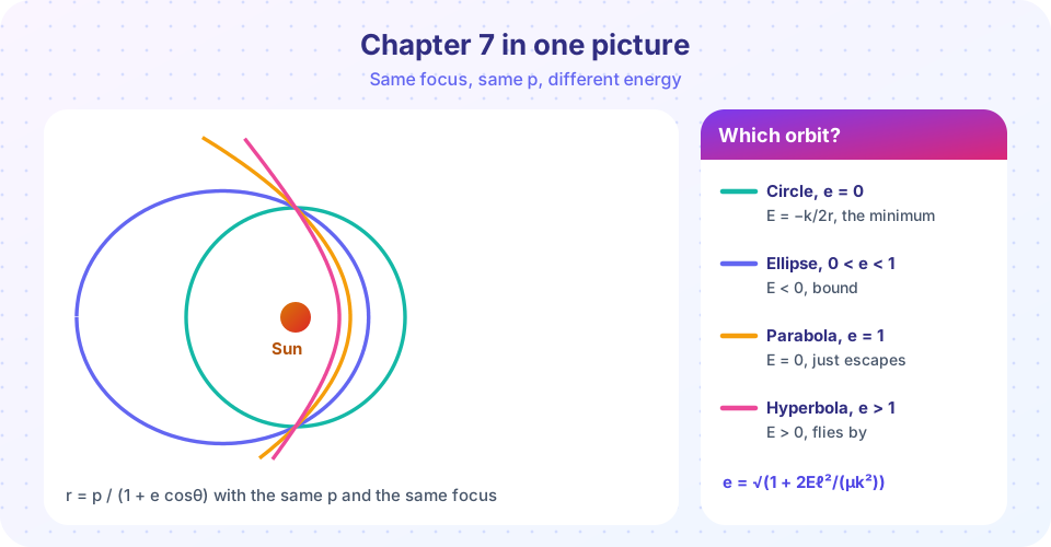
Recap table
| Step | Result |
|---|---|
| Reduce two bodies | one body of mass μ = m₁m₂/(m₁ + m₂) around a fixed center |
| Cyclic angle | ℓ = μr²θ̇ constant; dA/dt = ℓ/2μ |
| Effective potential | V_eff = ℓ²/(2μr²) + V(r), E = ½μṙ² + V_eff |
| Orbit equation | u'' + u = −μF(1/u)/(ℓ²u²), u = 1/r |
| Kepler orbit | r = p/(1 + e cosθ), p = ℓ²/μk, e = √(1 + 2Eℓ²/μk²) |
| Ellipse facts | a = −k/2E, T² = 4π²a³/G(m₁+m₂), v² = GM(2/r − 1/a) |
| Runge-Lenz | A = p × L − μk r̂ constant, magnitude μke |
Three habits to keep:
- Always ask which quantity is conserved (
E,ℓ, and for Kepler alsoA) before solving anything. - Read the effective-potential diagram first; it tells you the type of motion.
- Period depends on
aonly:T² ∝ a³for the same central mass.
An orbit classifier
Given a position r and speed v at one moment (with the velocity at an angle γ to the radius), you can find the whole orbit from conserved quantities. The TryIt below does it for a satellite near Earth: it computes the specific energy ε = v²/2 − GM/r and the specific angular momentum h = r v sinγ, then e, a, closest and farthest distance, and the period. GM for Earth is 3.986004418 × 10¹⁴ m³/s². The cases are textbook-style scenarios, not data of a real mission. An orbit with perigee below Earth's radius (6,371 km) would hit the ground: the code flags that.
Press Run (or Ctrl + Enter) to see the result here.
Program input · what you'd type while the program runs
Type the answers before you press Run, one per line. Each time the program reads a line (with input()), it gets the next line from this box.
Check your understanding
Quick check · 10 questions
of 10 answered You scored / 10 · perfect!
-
1. In the reduced one-body problem, the reduced mass of the Earth-Sun system is close to...
μ = m₁m₂/(m₁ + m₂) ≈ m_Earth when m_Sun ≫ m_Earth. -
2. Which conserved quantity gives Kepler's second law?
dA/dt = ℓ/(2μ) with ℓ constant. -
3. On the effective-potential diagram, an energy line meets the curve at two points. The motion is...
Two turning points r_min and r_max mean the radial motion oscillates between them. -
4. A body on a circular orbit sits where...
At the minimum, r cannot change. -
5. What is the eccentricity of an orbit with E = 0 under gravity?
e = √(1 + 2Eℓ²/μk²) = 1. -
6. A satellite's orbit has semi-major axis 4 times that of another around the same planet. Its period is...
T ∝ a^(3/2), so 4^(3/2) = 8. -
7. What is conserved in the Kepler problem but not in a general central force?
The Runge-Lenz vector is conserved only for the inverse-square force. -
8. The vis-viva equation lets you find speed from...
v² = GM(2/r − 1/a). -
9. For a force F = −k rⁿ circular orbits are stable if...
V_eff'' at the circular radius is proportional to 3 + n. -
10. Bertrand's theorem says closed orbits for all bound motions occur only for...
Only F ∝ 1/r² and F ∝ r have this property.
Summary
- Reduce, flatten, use
V_eff: that turns any central-force problem into a one-dimensional one. - For gravity,
Edecides the orbit: ellipse (E < 0), parabola (E = 0), hyperbola (E > 0). - Kepler's laws: ellipses, equal areas,
T² ∝ a³; the Runge-Lenz vector explains why orbits close.
Next: Chapter 8 overview: rigid bodies and small oscillations
Track your progress
Create a free account to tick off lessons and pick up where you left off on any device.
of Classical Mechanics: Lagrangian and Hamiltonian lessons completed